Modelling the Limit Order Book with an Eight-Variate Hawkes Process
Calibration, Stability and Endogeneity Analysis on Apple (AAPL) TAQ Data.
Published on: 10 Jun 2026
Note
This is a condensed write-up of a longer research project. Some images may take a while to load on this webpage.
Introduction
In recent years, there has been a surge in the use of limit order books (LOBs) in financial markets. This is largely due to technological advancements and access to real-time current states of the LOB which supply buyers and sellers with "the ultimate microscopic level of description". Modeling LOBs is vital as they provide information about the supply and demand, help measure market liquidity and aid algorithmic traders in using simulations to test their strategies without the risk of losing capital. Furthermore, LOB modeling is essential for quantifying price and market impact, illustrating how individual trades influence the aggregate state of the book and allowing participants to minimize their execution risk.
Essentially, the order book is a collection of all the available orders that have arrived at different time stamps. Hence modeling it as a Poisson queuing process is quite intuitive and common. These models are widely known as the zero intelligence model as they are not able to store any form of historical information or heuristics.
We calibrate an eight-variate Hawkes process to a full day of Apple top-of-book data, split into thirteen windows of 30 minutes each, and calculate the branching matrix and its spectral radius for each one of them. Furthermore, we then push the analysis one step further by exploiting the multitype Galton–Watson cluster representation of the calibrated Hawkes process to convert the abstract spectral radius into two key scalars. Firstly, the expected size of the event cascade triggered by a single immigrant of each type. Secondly, the proportion of all observed activity that is endogenously generated rather than driven by exogenous information. Four empirical findings emerge:
- a strikingly stable, near-critical spectral radius across the trading day
- a similarly high aggregate endogeneity (), calculated independently via cluster decomposition, which confirms that only about 5% of top-of-book events are exogenous arrivals.
- a dominant limit cancel () feedback loop as the principal channel of market reflexivity
- self-excitation of non-aggressive market orders consistent with the fragmentation of meta-orders
Furthermore its important to point out that four of the thirteen windows did not converge to the near critical minimum. However, we discuss that this is a calibration inconsistency rather than a change in the underlying properties of the order book.
Background
The crucial issue: A lack of endogeneity
Whilst we can make our Poisson models increasingly sophisticated and try capture more features, they all fundamentally lack one of the key market properties for microstructure modeling, they fail to capture market endogeneity. High frequency limit order books illustrate order clustering and memory properties. Whenever a massive market order arrives and consumes several price levels of the limit order book, it alters the state of the market. Such an event instantly triggers a chain of algorithmic reactions, Market makers will cancel their exposed limit orders to avoid adverse selection.
Conclusively, the key thing to note is that trade causes trade. Poisson process at their core assume that the arrival of an event does not change the probability of future events. They fail to account for the herd behavior, feedback loops and the cause and effect relationship. Hence in order to model such an environment we must look beyond independent increments and into the realm of self-exciting models.
The Self-Exciting Hawkes Process
We require a self-exciting counting process for our use case. We define it as a process where the occurrence of an event explicitly causes a temporary increase in the conditional intensity function . The hawkes process is the canonical self-exciting model. It is a counting process whose conditional intensity takes the specific form:
Here we use to denote the exogenous intensity, also known as the background intensity which represents the rate of arrival of independent arrivals. The excitation kernel function represents the positive influence all the past events at time exert on the current intensity at time . Illustrating the intensity as a stochastic integral with respect to the jump process, we are able to effectively capture the endogenous feedback loops that drive microstructure dynamics. Thus we are able to define a process that is able to produce the clustering, cross-excitation and short run feedback observed in real order flow.
Kernel Selection
The exponential kernel possesses the unique memoryless property which helps us out immensely for tractability:
This helps our activation function attain the key Markovian property required for computational optimization. We can exploit this property and manage a single state variable to record history. This allows us to calculate the log-likelihood in linear time. The key thing to note is that the exponential kernel is often the only mathematically tractable solution for MLE.
Despite the benefits of exponential kernel, some research has illustrated that the order-flow autocorrelation can often exhibit long-memory property. However, the power kernel comes with a great computational disadvantage. It does not possess the memoryless Markovian property. Hence we cannot segregate into and . This infers that calculating requires us summing over the entire history , presenting as a great computational challenge. For a dataset as big () as ours this would require trillions of operations for a single evaluation of the MLE and quadratic time complexity.
For the purpose of this research we will be utilizing the exponential kernel. Whilst we sacrifice the long-memory benefits of the power kernel we are guaranteed the computational tractability needed to process millions of limit order book events. Furthermore by restricting the parameter space to single matrices and , we achieve a clear Branching matrix , allowing us to conduct stability analysis.
Branching Ratio and Market Stability
Often we are concerned with the overall macroscopic performance of the asset. Hence, in order to analyse this we need to view the hawkes process as a branching process, specifically using an immigration-birth representation (also known as the Galton-Watson). Under this framework we divide the market events under two categories:
- Immigration events (Exogenous events): These are our foundational parent nodes of our branching process . These events arrive independently according to a Poisson process driven only by the background intensity, .
- Offspring (Endogenous Events): These are child nodes generated by our historical parent node at time . These nodes are generated by internal feedback loops of the market and maintained by the excitation kernel .
To judge the quality of the Apple stock we will need a metric to measure the market endogeneity, a measure of how much of the trading activity is self-generated rather than driven by exogenous events. For this we will be looking at the branching ratio , which represents the norm of the excitation kernel. For our exponential kernel it simplifies to a neat closed form ratio:
The value of the branching ratio can help us learn about the asset's market stability:
- stable (subcritical) region: This occurs when the value of the ratio implying that each parent produces on average less than one offspring. Hence the Galton-Watson tree eventually fades out.
- Unstable (supercritical) region: This occurs when the value of , indicating that each parent produces enough offspring to sustain growth indefinitely. This process becomes mathematically non-stationary, and results in an explosion of events to infinity. In terms of market terminology, it represents a market flash crash or a liquidity crisis.
How close sits to unity is itself a measure of how reflexive, how driven by its own past, the market is. An important point to note is empirical estimates on high-frequency data have repeatedly placed close to 1, suggesting modern markets operate near criticality.
Implementation / Methodology
The Microstructure Event Space
We decompose the limit order book in a discrete set of events. In high-frequency setting events that occur deep in the limit order book have very little informational value about the prices hence we will only be considering events that occur at level 1, the best buy and ask price. Hence we will adapt the framework introduced in Gašperov and Kostanjčar (2022), whereby the model has 8-dimensions. We define our multi-variate event space , consisting of 8 unique events as:
Events are distributed based on three categories:
- Order Type: Market Orders (M) consume liquidity, Limit Orders (L) introduce liquidity, and Cancellation (C) remove liquidity.
- Trade direction: Buy side () affect the bid side, whilst Sell side () affect the ask side.
- Aggressiveness: Lastly, aggressiveness, denoted by () indicates whether the volume of the event is large enough to consume the entire queue at level 1, and hence causing a shift in the mid price . On the other hand, a non-aggressive trade () does not alter the mid price.
The Multivariate Hawkes Process Intensity formulation
To model this 8-variate event space, we define an 8 variate counting process . The intensity of the -th event type at time is formulated as:
with exponential kernels . This multivariate equation contains three unique components that we will be calibrating using empirical data:
- The Exogenous Baseline Vector (): The vector represents the baseline intensities of each of the events defined earlier. This represents the independent arrival rate of orders based on exogenous factors.
- The Excitation Matrix (A): Each element provides a quantitative value illustrating the impact in the intensity of event caused by the occurrence of event . Diagonal entries measure self-excitation. Off-diagonal entries capture cross-excitation, such as , which records how an aggressive buy market order alters the subsequent rate of aggressive sell-side cancellations.
- The Decay Matrix (B): The matrix informs us about how quickly the market reduces the impact of past events. A high value of would indicate that the cross excitation is short lived.
The Cluster Representation and the Endogenous Activity Share
For a stable univariate Hawkes process with baseline intensity and branching ratio , each immigrant produces, on average, first-generation offspring, second-generation offspring, and so on. The expected total size of the Galton-Watson cluster started by a single immigrant is therefore:
Now we move on and generalize this theory to fit our eight variate framework. Here an immigrant of type produces descendants according to the multi-type Galton-Watson process, where the type distribution of offspring is dictated by the mean offspring matrix . Hence summing over all the generations will yield us the per type cluster matrix:
where the Neumann series converges by the Perron–Frobenius spectral condition . By weighting all the different event types by their long-run intensities, we arrive at the aggregate endogeneity:
It restricts between 0 (a pure, entirely exogenous Poisson process where ) and 1 (a completely self-sustaining process with no outside input, ). All in all, its a useful metric that helps provide us with a single scalar summary of market reflexivity, which can be interpreted as a total percentage of order book activity that is internally generated.
Calibration and Optimization
In order to make sure our model is embedded in empirical data we need to calibrate the parameters . The most popular way to do this is through Maximum likelihood estimation. The log-likelihood function is given by:
The first term rewards the model for assigning a high intensity at the times and types where events were actually observed. Whilst the second term penalizes any intensity assigned to event types that did not in fact arrive, and prevents the optimiser from inflating uniformly to maximize the first sum.
However one of the key drawbacks of estimating parameters using the log-likelihood is that while its statistically sound, it is computationally expensive scaling quadratically. This is where the strength of choosing an exponential kernel is illustrated. Due to its memoryless property we can maintain a recursive state variable to store the history, and update it at each iteration. Following Ozaki (1979), we define:
Between two consecutive arrivals the state decays exponentially at the channel-specific rate; immediately after the -th event the column corresponding to its type is incremented by one. The full likelihood is therefore evaluated in , which on our data brings a single likelihood call from intractable to a small number of seconds. We pass this function to the L-BFGS-B optimization routine (a quasi-Newton optimiser well suited to bound-constrained smooth objectives) to iteratively find the global maximum.
Analysis
We tuned the parameters of the 8-variate hawkes model using L-BFGS-B optimization on Apple's consolidated trade and quotes data, the dataset contained about 2 million top of the book events of a single day. We made use of the Lee-Ready algorithm to conduct trade sign inference. We split the whole trading day into 13 separate windows of 30 minutes.
Intraday Stability
We were able to attain good calibration across nine of the windows with the mean value of and a standard deviation of 0.0002. Furthermore, its vital to note that all the windows are within the stable requirement of , indicating that our process is in sub-critical state.
| Window | N events | Status | |
|---|---|---|---|
| 09:30–10:00 | 269 948 | 0.9502 | converged |
| 10:30–11:00 | 344 646 | 0.9501 | converged |
| 12:00–12:30 | 234 434 | 0.9502 | converged |
| 12:30–13:00 | 203 340 | 0.9502 | converged |
| 13:00–13:30 | 226 922 | 0.9505 | converged |
| 13:30–14:00 | 227 295 | 0.9505 | converged |
| 14:00–14:30 | 291 775 | 0.9505 | converged |
| 15:00–15:30 | 341 702 | 0.9501 | converged |
| 15:30–16:00 | 348 710 | 0.9502 | converged |
| Mean (converged) | — | 0.9503 | — |
| Std. dev. (converged) | — | 0.0002 | — |
| 10:00–10:30 | 404 515 | 0.1107 | anomalous |
| 11:00–11:30 | 238 056 | 0.3337 | anomalous |
| 11:30–12:00 | 243 694 | 0.3575 | anomalous |
| 14:30–15:00 | 281 051 | 0.2704 | anomalous |
The intriguing feature we discover through the table is not that the values of the different windows are in obedience with theory, but rather the fact that despite there being significant difference in event counts across the windows, the individual being quite different across all windows the spectral radius is quite invariant. This signals just the strength of the scalar value in demonstrating the dynamics of the entire limit order book.
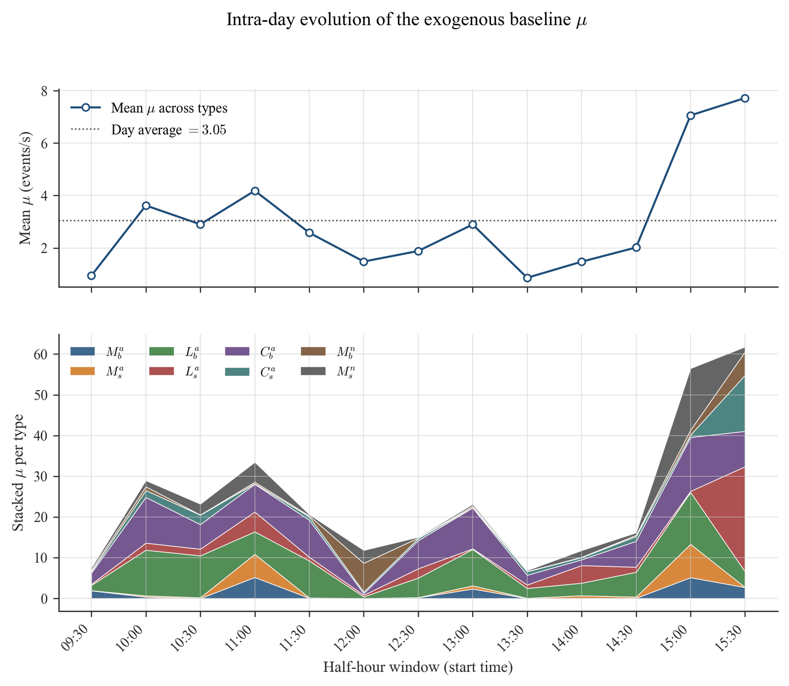
Intraday evolution of the exogenous baseline intensity . Top: the mean baseline rate across the eight event types per half-hour window. Bottom: the per-type stack, with one band per event type. Both panels show the same intraday U-shape in absolute exogenous activity — high at the open and close, depressed through the lunch window — that is conspicuously absent from the spectral-radius profile.
Whilst the background intensity of the market changes throughout the day the endogenous reflexive structure, depicted with the help of , is mostly constant.
Branching Matrix
The figure below illustrates the calibrated branching matrices for our nine converged windows. Upon observing, its clear they all share the same qualitative structure. They all have a strong self-exciting market order diagonal, in tandem with dominant off-diagonal link between the limit orders and cancellations (), common across all the nine matrices. In contrast, the matrices of the four anomalous windows lack this structure.
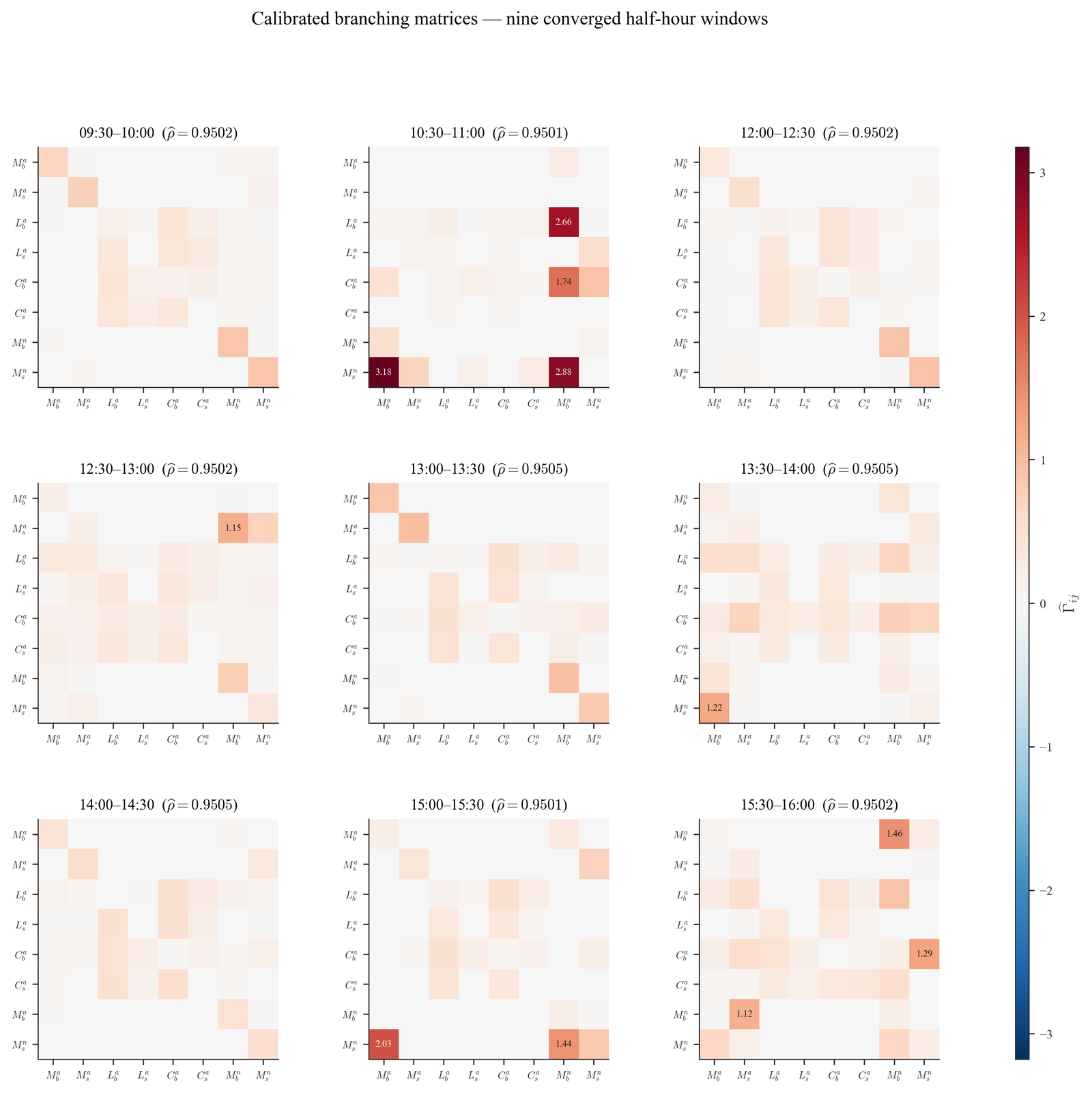
Calibrated branching matrices for the nine converged half-hour windows, plotted on a shared colour scale. Each panel is titled with the window's time range and its spectral radius . The dominant feedback block on the aggressive side of the book and the diagonal market-order self-excitation are visually consistent across all nine panels.
Taking the opening 09:30–10:00 window without a loss of generality, we can segregate all the self-exciting endogenous events into separate groups. Firstly, the aggressive market cluster: , . Secondly the non-aggressive market clusters: , . The passive buy side limit-order and cancellation diagonals are an order of magnitude smaller. Moreover, there is a feedback loop between limit orders and cancellations , . Lastly, its important to note that there is negligible cross-excitation between aggressive buy and aggressive sell market orders () implying that they essentially operate independently.
Triggers and Reactions
Summing over the column values of the branching matrix provides us with the expected number of offspring events that will be generated by a single event of each type. The row sum value provides us with the expected number of times this event occurs from all other types.
| Event type | Column sum (triggers) | Row sum (reacts) |
|---|---|---|
| 0.814 | 0.875 | |
| 0.904 | 0.923 | |
| 1.310 | 1.033 | |
| 0.483 | 1.132 | |
| 1.331 | 1.059 | |
| 0.683 | 1.114 | |
| 1.258 | 1.000 | |
| 1.288 | 0.935 |
Cancellations and limit orders illustrate the most profound impact. A single aggressive buy cancellation triggers approximately 1.33 events, whereas a single aggressive buy market order only produces about 0.81. The column sum values of cancellations and limit orders illustrate that liquidity provision and withdrawal events provide more information to the book in high frequency setting than others. This claim is further supported by Cont et al., who illustrate that majority of the price changes in S&P 500 can be through the imbalance of limit orders and cancellations, without considering the actual trade. Lastly, the Buy-side events (, ) carry more triggering power than the corresponding sell-side events.
Cluster Sizes and the Endogenous Activity Share
| Window | |||
|---|---|---|---|
| 09:30–10:00 | 0.9502 | 0.965 | 28.80 |
| 10:30–11:00 | 0.9501 | 0.920 | 12.43 |
| 12:00–12:30 | 0.9502 | 0.981 | 53.35 |
| 12:30–13:00 | 0.9502 | 0.914 | 11.66 |
| 13:00–13:30 | 0.9505 | 0.947 | 18.83 |
| 13:30–14:00 | 0.9505 | 0.948 | 19.22 |
| 14:00–14:30 | 0.9505 | 0.952 | 20.67 |
| 15:00–15:30 | 0.9501 | 0.986 | 73.24 |
| 15:30–16:00 | 0.9502 | 0.973 | 36.47 |
| Mean | 0.9503 | 0.954 | 30.5 |
The aggregate endogeneity proportion is averaged across the nine converged windows. This is in agreement with spectral radius , and hence consistent with the theoretical expectation of in the multivariate setting. It means, that about 95% of all top-of-book events on Apple are endogenously triggered by previous events, and only 5% are truly exogenous arrivals from outside the book. Confirming the hypothesis that majority of order activity throughout the day in Apple's book feeds on itself.
The per-type endogeneity depicts that nearly every event type is extremely endogenous (seven of eight have ), the single mild outlier is the aggressive buy market order at 0.846. This reveals a distinct asymmetry: aggressive buy market arrivals carry a slightly larger exogenous component than their sell-side or non-aggressive counterparts. Hence, the cluster decomposition provides us with a new independent line of evidence that further solidifies our understanding of the structure of the order book. It precisely confirms the findings mentioned in the spectral radius and the branching matrix entries: a near critical almost fully endogenous reflexive system whose dominant excitation channels are limit-order placement, cancellation, and metaorder fragmentation on the buy side of the book.
The Four Anomalous Windows
Four of the thirteen windows converged to relatively low spectral radius values, illustrating that the L-BFGS-B routine converged to a secondary basin of the multi-modal log likelihood function. Three observations identify this as a calibration issue rather than a genuine market regime change:
- Disproportionate runtime: On similar event counts (– events), a thirty minute time block takes about 2–5 hours to converge, whereas these 4 windows took up to 15 hours to converge. Such disproportionate runtime along with vastly different parameters indicates the algorithm was traversing flat regions of a non-convex surface, which resulted in it settling into a shallow local mode rather than the global maximum.
- Loss of structural integrity in : Among all the valid windows the branching matrices illustrate a clear limit-cancel feedback loop. However, in these 4 anomalous windows the loop is non-existent, instead we have a matrix of scattered values. Such lack of structure suggests that the results are not a real market shift, rather a systematic error.
- Alignment with independent literature: Filimonov and Sornette have already explored such shortcomings of utilizing hawkes models on stock data. They discuss that the log-likelihood is often multi-modal, having multiple peaks, where we have one true basin near the true near-critical solution and multiple other basins that the optimizer may converge to depending on its start. They highlight that single-start MLE on such surfaces can produce estimates that are biased downwards by an order of magnitude.
Thus, we exclude these 4 windows from our analysis and focus on the remaining nine as our calibration. This is done because re-running the four windows under different initialization to achieve near-critical estimates would have an adverse impact on the independence of our results: our results would be partly engineered to meet our desired outcome.
Conclusion
Limitations and Improvements
Kernel Specification. As discussed earlier the exponential kernel decays at a geometric rate, however literature illustrates that the autocorrelation of signed order flow in markets decays algebraically. Furthermore, Hardiman et al. also depicted that when we try to fit a short term memory kernel in settings where long term memory kernels are required the estimates we get for the branching ratio tend to be biased downwards. This would infer that the value we obtain is truly a conservative lower bound for the real value of market endogeneity in Apple's data. Thus, a natural extension to our current pipeline can be to fit a power-law or power-law with cutoff kernel using non-parametric estimators in a way that's computationally feasible. Specifically, one can implement a piecewise-exponential kernel to approximate a power-law structure.
Multi-modal likelihood and basin identification. A multivariate hawkes process's log likelihood surface with this many parameters is known to be multi-modal, where each basin results in different estimates. Hence a single run of the L-BFGS-B algorithm can result in it converging to a local basin, and not the global maximum. Two of the most direct remedies to this problem would be, firstly to use a multi-start MLE: where we would run the algorithm from several initializations and in the end pick the one with the highest likelihood. Alternatively, the EM algorithm could be employed to resolve this challenge.
Analytic Gradient. We are currently deploying the finite difference technique to calculate the gradients of the log likelihood function for all of our 136 parameters individually. A potential improvement could be to analytically calculate the gradients.