Deployment of a Machine Learning pipeline to Predict House Prices using ZenML
This project trains and deploys a machine learning pipeline to predict house prices using ZenML
Published on: 6/8/2024
Note
The code for this project can be found on GitHub. The code is fully documented. Some images may take a while to load on this webpage.
Introduction
This project aims to analyze the data from Kaggle. The goal of this project is to build a model to predict the price of the house based on the features provided in the dataset. This project has been built using ZenML. ZenML is an MLOps framework that helps you to build, train, and deploy machine learning models. We First conduct EDA (Exploratory Data Analysis) to understand the data and then build a model to predict the price of the house. Then run the pipeline to train the model and deploy it. Porject built using such frameworks help in transforming industries by bridging the gap between data science and operations, allowing companies to efficiently deploy, monitor, and manage machine learning models at scale.
Background/Implementation
Data
We are using the dataset from the Kaggle. The dataset contains the following columns:
- price (type:int64) : Price of the house
- area (type:int64): Area of the house
- bedrooms (type:int64): Number of bedrooms
- bathrooms (type:int64): Number of bathrooms
- stories (type:int64): Number of stories
- mainroad (type:object): Whether the house is on the main road or not (categorical: yes/no)
- guestroom (type:object): Whether the house has a guest room or not (categorical: yes/no)
- basement (type:object): Whether the house has a basement or not (categorical: yes/no)
- hotwaterheating (type:object): Whether the house has hot water heating or not (categorical: yes/no)
- airconditioning(type:object): Whether the house has air conditioning or not (categorical: yes/no)
- parking (type:int64): Number of parking spaces
- prefarea (type:object): Whether the house has a preferred area or not (categorical: yes/no)
- furnishingstatus (type:object): Furnishing status of the house (categorical: furnished, semi-furnished, unfurnished)
EDA
We first conduct EDA to understand the data. We check for missing values, check the distribution of the data, and check the correlation between the features. When we run the following code, we find out that there are no missing values in the dataset.
print(df.isnull().sum())
Using the following code, we check the distribution of the data.
  class NumericalUniVarientAnalysis(UnivariateAnalysisTemplate):
    def univariate_analysis(self, df: pd.DataFrame, feature: str):
        plt.figure(figsize=(12, 8))
        sns.histplot(df[feature], kde=True, bins=30)
        # kenel density estimation a smooth version of the histogram
        plt.title(f"{feature} Distribution")
        plt.xlabel(feature)
        plt.ylabel("Frequency")
        plt.show()
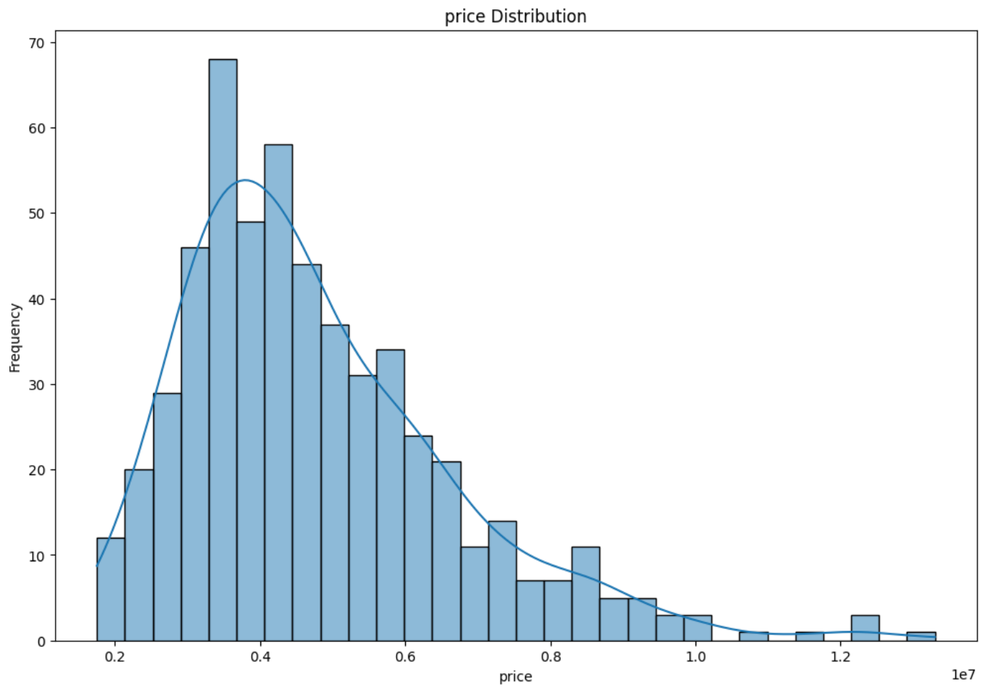
price distribution
As it is evident from the above plot, the price is right-skewed. This infers that majority of the houses are priced lower than the mean price. Its because of a few houses that are priced very high, the mean price is higher than the median price. We will handle this skewness later in the pipeline, using the log transformation.
We can also observe the correlation heatMap between the different numerical features.
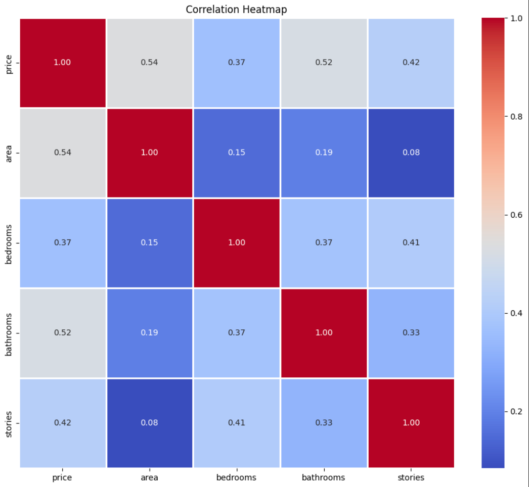
correlation heatmap
From the above heatmap, we can observe that the highest correlation is between price and area of 0.54. This inferes that the price of the house and the area of the house are positively correlated. However the overall correlation between the features is not very high. This would mean that using reguralization techniques like Lasso and Ridge would not be very useful, there performace would be similar to the linear regression model.
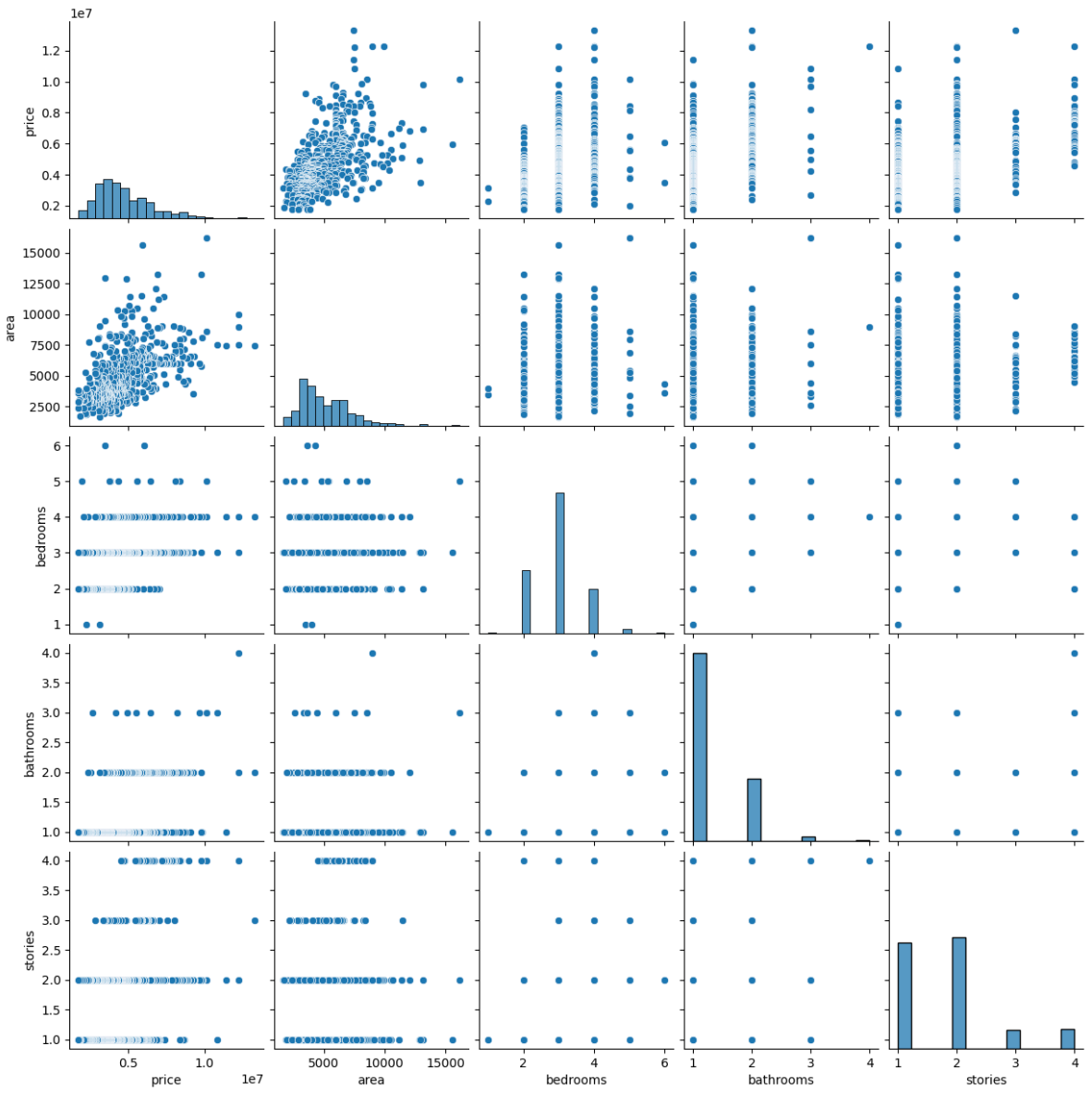
pairplot
The pairplot shows the relationship between the different numerical features. We can observe that the price of the house is positively correlated with the area of the house. However, the isnt a correlation between the price of the house and the number of bedrooms, bathrooms, and stories. We can also observe the histogram of bedrooms and stories and infer that most of the houses have 2-3 bedrooms while there are very few properties with 6 bedrooms or 4 stories.
Methodology/Implementation
This project has been built using ZenML, so the implementation is divided into steps within a ZenML pipeline. We run the run_deployment.py script to execute the pipeline. The continuous deployment pipeline is set up in a way that ZenML monitors for changes and responds accordingly. The continuous pipeline includes the following steps:
- Running the training pipeline
- Making a deployment decision
- Deploying the model
The training pipeline has the following steps:
- Data Ingestion: Load raw house pricing data from a zip file.
- Feature Engineering: Apply specified transformations (e.g., log transformations) on selected features.
- Outlier Detection: Detect and remove outliers from the dataset based on the 'price' column.
- Data Splitting: Split the cleaned data into training and test sets.
- Model Building: Train four different models:
- Linear Regression
- Polynomial Regression
- Ridge Regression
- Decision Tree Regression
- Model Evaluation: Evaluate each model on the test dataset using predefined metrics.
In order for the pipeline to run successfully, we need out stack to look like this:
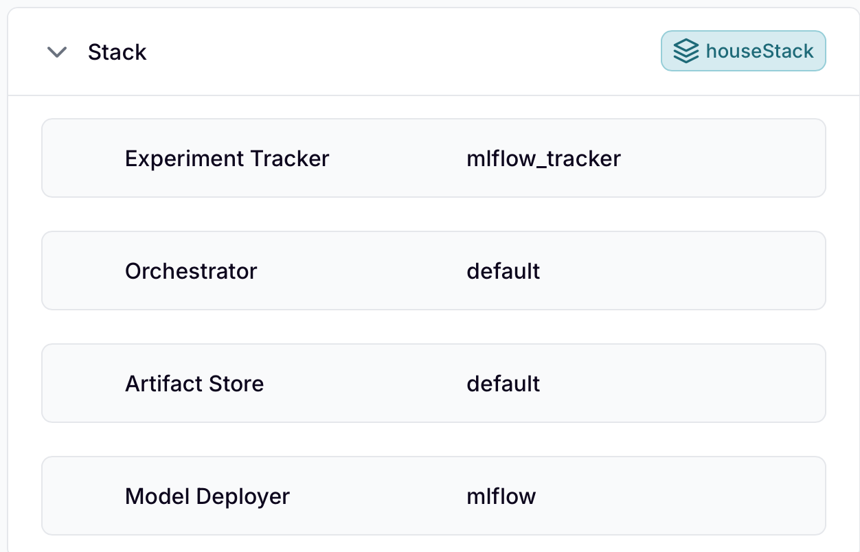
stack
The stack consists of the following components:
- Experiment Tracker: Tracks and manages the experiments you run during the development of your machine learning models. Logs experiment runs, metrics, and artifacts.
- Orchestrator: Manages the pipeline runs. It is responsible for scheduling and executing the pipeline steps in the correct order.
- Artifact Store: A storage location for the artifacts generated during the pipeline runs, such as the trained models, datasets, and evaluation metrics.
- Model Deployer: Automates the deployment of the trained models to the desired deployment target.
Analysis
We have trained four different models, the results of the models are as follows:
-
Linear Regression:
- Mean Squared Error: 0.0735098183459159
- R2 Score: 0.6185705760818005
-
Polynomial Regression:
- Mean Squared Error: 0.08465818180067468
- R2 Score: 0.5607236932318227
-
Ridge Regression:
- Mean Squared Error: 0.08467847967370172
- R2 Score: 0.560618371164789
-
Decision Tree Regression:
- Mean Squared Error: 0.08822839405952121
- R2 Score: 0.5421984943427525
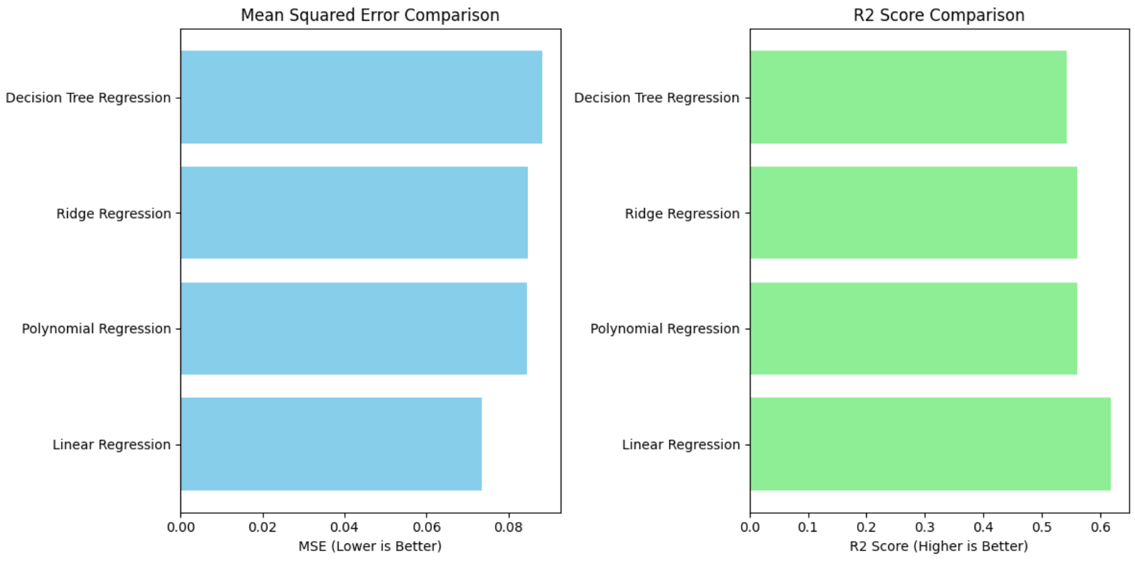
model comparison
Mean square error is the average of the square of the errors. The smaller the mean square error, the better the model. The R2 score is the proportion of the variance in the dependent variable that is predictable from the independent variable. The R2 score ranges from 0 to 1. The closer the R2 score is to 1, the better the model. From the above results, we can infer that the Linear Regression model has the lowest mean square error and the highest R2 score. Thus, Linear Regression model performs the best in terms of MSE and R2 score.
Conclusion
In conclusion, this project has successfully trained and deployed a machine learning model to predict house prices using ZenML. The project has been built using ZenML, an MLOps framework that helps you to build, train, and deploy machine learning models. The project has successfully trained four different models and evaluated them based on predefined metrics. The Linear Regression model has been identified as the best model among the four models based on the mean square error and R2 score. The project has successfully deployed the Linear Regression model. The project has successfully trained and deployed a machine learning model to predict house prices using ZenML.