Learning Sparse Sentence Encoding without Supervision: An Exploration of Sparsity in Variational Autoencoders

Here we discuss the following paper: Learning Sparse Sentence Encodings without Supervision by Victor Prokhorov, Yingzhen Li, Ehsan Shareghi, and Nigel Collier.

The paper begins by discussing a problem: when we represent a sentence as a fixed-length vector (an embedding), it turns out to be very dense. This means that most of the values in the vector are non-zero.

To give an example, imagine the following sentence for sentiment analysis: “I love this movie”

A 5-dimensional (5D) vector may look something like this:

1[0.23, -1.12, 0.55, 0.66, -0.34]

So if you have a 768-dimensional BERT embedding, you might see something like:

1[0.11, -0.04, 0.92, 0.00, -0.33, 0.07, … , -0.15]

The paper proposes the idea of sparse sentence vectors. A sparse vector is the opposite of dense: most entries are exactly zero, and only a few are non-zero.

• Dense sentence embedding:

  1[0.3, -0.1, 0.5, 0.2, -0.4, 0.1, 0.6, -0.2, 0.3, 0.05]

• Sparse sentence embedding:

  1[0, 0, 1.2, 0, 0, 0, -0.9, 0, 0, 0]

The main reasons why we should do this are:

1. Firstly, each sentence encodes a different meaning, emotion, topic, style, etc., so different subsets of dimensions should be used for different types of sentences, instead of every dimension being used for all.
2. Secondly, sparse representations are often easier to interpret and can be more efficient.

The paper learns such encodings using unsupervised learning, specifically Variational Autoencoders (VAEs).

VAE Background

A VAE is a probabilistic autoencoder. To understand this, it's important to first understand how a classical autoencoder works.

In a classical autoencoder, there are 2 key parts:

• Encoder: In this part, we take the input (a sentence in our case) and map it to a "code" (a vector of numbers).
• Decoder: In this bit, we take the above vector and try to reconstruct the original input.

So if the input sentence is: “The movie was surprisingly good,” the autoencoder might:

• Encoder → code:

  1[0.3, -1.1, 0.8]

• Decoder → tries to regenerate: “The movie was surprisingly good.”
• Training: Adjust parameters so reconstructions match inputs as closely as possible.

Probabilistic Autoencoders (VAEs)

A VAE is probabilistic instead of deterministic.

• Instead of the encoder outputting a single vector, it outputs a distribution over possible vectors.
• Instead of the decoder outputting a single sentence, it outputs a distribution over possible sentences.

For each input sentence $x$, the encoder neural network produces two vectors: $\mu(x)$ and $\sigma(x)$. We treat these as the parameters of a multivariate normal (Gaussian) distribution over the latent code $z$:

• Mean: $\mu(x)$
• Variance per dimension: $\sigma(x)^2$
• (Typically no covariance between dimensions)

During training, we sample $z$ from this Gaussian and feed it to the decoder.

In the training process, we try to maximize the Evidence Lower Bound (ELBO):

$L(\theta, \phi; x) = \mathbb{E}_{q_{\phi}(z|x)}[\log p_{\theta}(x|z)] - D_{KL}(q_{\phi}(z|x) \mid\mid p_{\theta}(z))$

The second term is the KL divergence ($D_{KL}$), which measures how different two probability distributions are. This term acts as a regularizer. It forces the learned distribution $q_{\phi}(z|x)$ (the "posterior") to be close to a predefined "prior" distribution $p_{\theta}(z)$ (usually a standard normal distribution). This helps structure the latent space and prevents the model from simply memorizing the data.

The Paper's Contribution: HSVAE

The paper introduces a new extension called HSVAE (Hierarchical Sparse VAE) to enforce sparsity. This model extends a standard text VAE by replacing the simple Gaussian prior with a spike-and-slab prior.

Here's how it works:

1. Each latent dimension $z_i$ is drawn from a mixture of two Gaussians:
   • A "spike": A Gaussian with near-zero variance (e.g., $\mathcal{N}(0, 0.01)$). Dimensions drawn from this are effectively zero.
   • A "slab": A wide Gaussian with large variance (e.g., $\mathcal{N}(0, 1)$). Dimensions drawn from this are active and non-zero.
2. This "spike-vs-slab" choice is controlled by a higher-level latent variable $\gamma$.
3. For each dimension $i$, a variable $\gamma_i$ is drawn from a Beta distribution: $\gamma_i \sim \text{Beta}(\alpha,\beta)$. This $\gamma_i$ acts as the mixture weight between spike and slab: when $\gamma_i$ is large, the spike is more likely to be chosen, when small, the slab is more likely.
4. By choosing the Beta prior's parameters ($\alpha$ and $\beta$), the model gets a clean, probabilistic handle on how sparse the latent vector $z$ should be.

To measure how sparse the resulting vectors are, the paper uses Hoyer’s measure.

Performance/Result

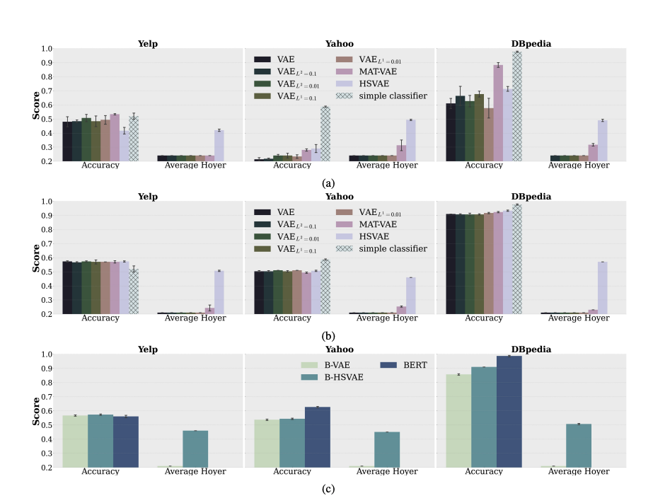
The paper uses the above image to illustrate the results. 3 different datasets are used to assess HSVAE. Each panel has two groups of bars, firstly is an Accuracy section this is used to identify how well a classifier the classifiers built on top of the embeddings predict the label. Second, is the Average Hoyer, used to quantify the sparsity of the latent vector. Where a higher value means more sparsity. Subfigure a is when the latent space is small (eg 32D). Subfigure b displays the results when the latent space is large (768D). And c is when the encoder is BERT-based instead of GRU.

Overall, the results show that HSVAE’s sparse latent codes (embeddings) perform about as well as the dense codes from regular VAEs. In smaller latent spaces HSVAE sometimes lags a bit behind, but with larger latent dimensions (768D) the performance of all VAE models becomes very similar.