Vision Transformer for CIFAR10 Classification

Note

The code for this project can be found on GitHub. The code is fully documented. Some images may take a while to load on this webpage.

Introduction

This post dives deeper into the vision Transformer model created to classify the CIFAR10 (Canadian Institute For Advanced Research) dataset. The CIFAR10 dataset is a dataset that contains 50,000 32x32 color images in 10 different classes. The dataset is split into 40,000 training images and 10,000 validation images. The model was trained on the training set and evaluated on the val set. The model was able to achieve an accuracy of 82.14 % on the validation set. The model was trained using the adam optimizer for 10 epoches. The idea of a vision Transformer comes from the paper "AN IMAGE IS WORTH 16X16 WORDS: TRANSFORMERS FOR IMAGE RECOGNITION AT SCALE" by Alexey Dosovitskiy.

The application of Vision Transformers (ViTs) in image classification is an important advancement in the field of computer vision, with significant real-world applications across various industries. With real-world applications in fields such as healthcare, autonomous vehicles, and security.

Background/Implementation

Its important to understand the idea of a transformer before understanding the vision transformer. below is a brief overview of the transformer architecture:

Transofrmer

We will use the transformer encoder block in this project as proposed in the paper "an Image is worth 16x16 words: transformers for image recognition at scale". The concept of the transformer architecture was introduced in the "attention is all you need" paper. In essence, The transformer encoder block is made up of two sublayers: a multi-head self-attention mechanism and a feedforward neural network. The multi-head self-attention mechanism is used to capture the relationships between the different tokens (in our case patches) in the input sequence. The feedforward neural network is used to process the output of the multi-head self-attention mechanism.

The self-attention mechanism allows the model to weigh the importance of each patch in relation to other patches. It consists of three main components: the query, key, and value. These are linear transformations of the input tensor.

The query represents what a patch is trying to understand or focus on. The key represents the relevant information that can help other patches focus on this patch. The value represents the actual information contained in the patch. To compute attention, we take the dot product of a patch's query with another patch's key. This gives us an attention score, which reflects how much one patch should attend to another. We compute this for all pairs of patches. The higher the attention score, the more "related" or relevant the patches are. For example, the dot product between two vectors will be higher when they point in the same direction, indicating strong correlation.

In the multi-head attention mechanism, instead of calculating attention just once, we compute it multiple times in parallel using different "heads." Each head learns different patterns or relationships between the patches, allowing the model to capture various types of information. Afterward, the outputs of all heads are combined to form the final attention result.

The following is the implementation of the self-attention mechanism in the transformer encoder block: For easier understading say we input a tensor of shape (1, 5, 128) where 1 is the batch size, 5 is the number of patches, and 128 is the embedding size.

class SelfAttention(nn.Module):

    def __init__(self, n_embd, n_head=4):
        super().__init__()
        assert n_embd % n_head == 0
        self.c_attn = nn.Linear(n_embd, 3 * n_embd)
        self.c_proj = nn.Linear(n_embd, n_embd)
        self.c_proj.NANOGPT_SCALE_INIT = 1
        self.n_head = n_head
        self.n_embd = n_embd

    def forward(self, x):
        B, T, C = x.size()
        qkv = self.c_attn(x)
        q,k,v = qkv.split(self.n_embd, dim=2)
        # We view qkv as Batch size, number of self-attention heads, T(sequence length), and number of dimensions per head
        q = q.view(B, T, self.n_head, C // self.n_head).transpose(1,2)
        k = k.view(B, T, self.n_head, C // self.n_head).transpose(1,2)
        v = v.view(B, T, self.n_head, C // self.n_head).transpose(1,2)
        att = (q @ k.transpose(-2, -1)) * (1.0 / math.sqrt(k.size(-1)))
        att = F.softmax(att, dim=-1) # convert the attention scores into probabilites
        y = att @ v # (B, h, hs, hs) * (B, h, hs, hs) -> (B, nh, T, hs)
        # After computing the attention output for each head, the heads are combined back into the original embedding dimension by reshaping:
        y = y.transpose(1, 2).contiguous().view(B, T, C)
        y = self.c_proj(y)
        return y

The tensor is passed through a linear layer to get the query, key, and value. The query, key, and value are then reshaped to have the shape (1, 5, 4, 32). The query, key, and value are then transposed to have the shape (1, 4, 5, 32). The query is then multiplied by the transpose of the key and then divided by the square root of the key size (regularization). The result is then passed through a softmax function to get the attention scores. The attention scores are then multiplied by the value to get the output tensor. The output tensor is then reshaped to have the shape (1, 5, 128) and passed through a linear layer to get the final result.

The following is the entire implemenation of the tranfromer block:

class Block(nn.Module):
    def __init__(self, n_embd):
        super().__init__()
        self.ln1 =  nn.LayerNorm(n_embd)
        self.attn = SelfAttention(n_embd)
        self.ln2 =  nn.LayerNorm(n_embd)
        self.mlp  = MLP(n_embd)

    def forward(self, x):
        x = x + self.attn(self.ln1(x)) # residual connections
        x = x + self.mlp (self.ln2(x))
        return x

As it can be seen in the forward method, the input tensor is passed through a layer normalization, then passed through the self-attention mechanism, after which we have a residual connection. We need residual connections to tackle issues like the vanishing gradient problem and stability, which occur while training deep networks. The output of the self-attention mechanism is then passed through another layer normalization layer, then passed through a feedforward neural network, after which we have another residual connection. The output is then returned.

Vision Transformer

The idea of a vision Tranformer is quite simple. Instead of using CNNs, we can use a transformer to process images. In a simple decoder only tranformer (used in NLP), the transformer is fed a sequence of tokens then the transformer processes the sequence of tokens. Similarly, in a vision transformer, the image is divided into patches and each patch is treated as a token. The patches are then flattened and fed into the transformer.

using the folllowing code:

  class PatchEmbedding(nn.Module):
      def __init__(self, in_channels=3, patch_size=4, emb_size=16):
          super().__init__()
          self.patch_size = patch_size
          self.projection = nn.Sequential(
              nn.Linear(patch_size * patch_size * in_channels, emb_size)
              )
      def forward(self, x):
          x = rearrange(x, 'b c (h p1) (w p2) -> b (h w) (p1 p2 c)', p1=self.patch_size, p2=self.patch_size)
          x = self.projection(x)
          return x

Fristly, we get patch embeddings by dividing the image into patches and then flattening them. The patches are then passed through a linear layer to get the patch embeddings of our desired embedding size. The tensor returned now is of 3 dimensions: batch size, number of patches, and embedding size.

Based on the paper we also need a CLS token (classification token). The CLS token is a learnable parameter that is added to the patch embeddings. This is done because the cls token acts as a placeholder that interacts with all the other patches, which would make sure the output vector has information from all the patches.

After concatinating the cls token with the patch embeddings, we add positional encodings to the patch embeddings. The positional encodings are added to the patch embeddings to give the model information about the spatial information of the patches. The positional encodings are added to the patch embeddings and then passed through the transformer. Patch embeddings contain information about the content of the patch, while positional encodings contain information about the spatial information of the patches.

        x = torch.cat([cls_tokens, x], dim=1)
        x += self.positional_emb[:, :(T + 1)]

Following this you just pass x into the transformer.

training the model

To train the model we used adam optimizer, and used the Cosine Annealing Learning Rate Decay. The model was trained for 10 epoches.

Analysis/Results

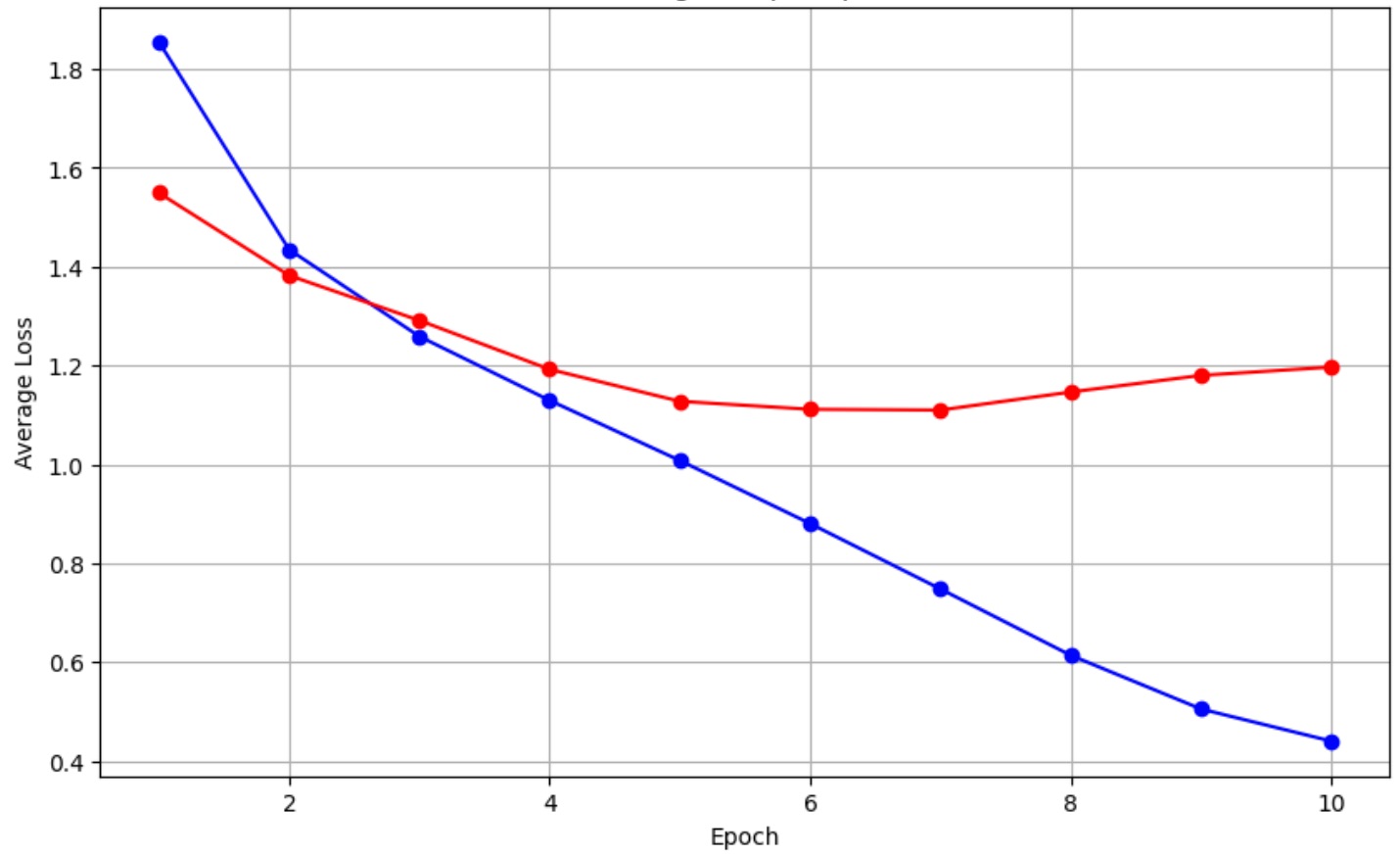
After training the model for 10 epoches, the model achieved an accuracy of 82.14 % on the validation training set. The validation loss further could be used to fine-tune the hyperparameters of the model, as it should be. However due to limited computer units on google colab, that was not done. Follwoing is the training and validation loss graph:

The one in the blue is training loss and the one in the red is validation loss.

Firstly, it is visible that the training loss does decreases over the course of 10 epoches. The validation loss also decreases. However, after the 7th epoch, the validation loss starts to increase. This is a sign of overfitting. The model is starting to memorize the training data and is not generalizing well on the validation data. This could be due to the model being too complex or the model being trained for too long. The final validation loss is 1.2 and the final training loss is 0.44. The model could be fine-tuned by changing the hyperparameters of the model or by using techniques like dropout to prevent overfitting.

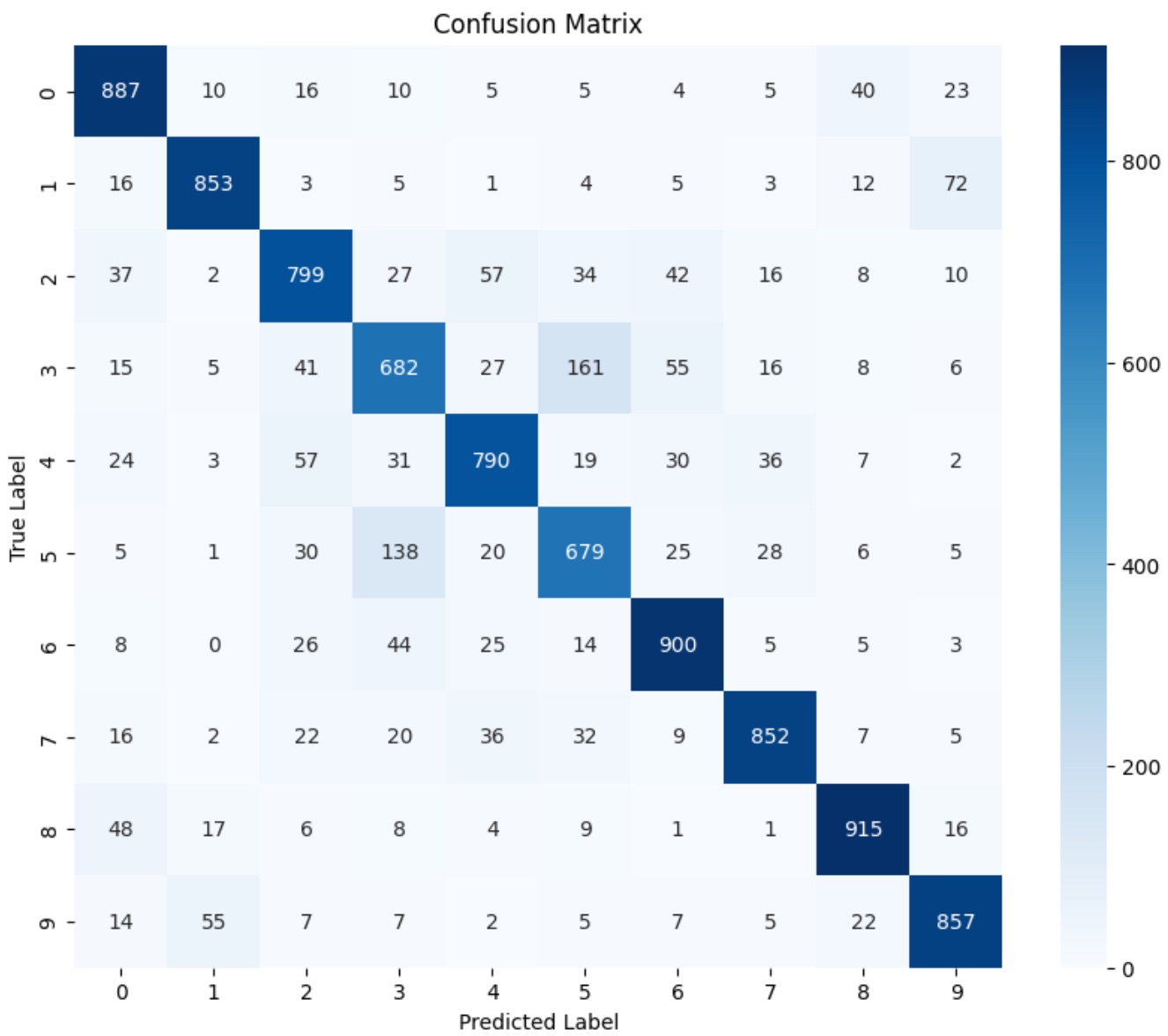
Below is the confusion matrix of the model:

The confusion matrix shows the number of correct and incorrect predictions made by the model. If we observe the matrix, it is visible that the model misclassfies the 3rd and the 5th class the most. When the actual label was 3, the model predicted 5 161 times, the highest misclassificaiton. Furthurmore, when the true label was 5, the model predicted 3 138 times. This high confusion between the two classes may indicate that their feature representations in the latent space overlap significantly, leading the model to make frequent errors between them. This issue could be mitigated by increasing the number of training samples for these classes or by using techniques like data augmentation to increase the diversity of the training data. As suggest before, regularization techniques like dropout could also help in tackling this issue.

Future Plans

This model was trained on the CIFAR10 dataset. The CIFAR10 dataset is a small dataset with low resolution images. This model was chosen to train on this dataset as it would be computational more feasible on google colab. However, the plan is train the same model on more complex datasets, datasets with a a large number of datapoints and higher resolution images. The model could be trained on datasets like the GTSRB (German Traffic Sign Recognition Benchmark), and others, such as ImageNet or CIFAR100. Then the results could be compared to see how the model performance changes with different datasets. If the performance decreases, we could investigate whether there is a correlation between factors such as dataset size, image resolution, or the complexity of the images. Additionally, it could provide insights into whether the model architecture needs to be adjusted, or if more data-specific augmentation, preprocessing, or regularization techniques are necessary to handle the increased complexity of the new datasets.

Conclusion

In conclusion, the vision transformer model was able to achieve an accuracy of 82.14 % on the validation set. The model was trained for 10 epoches and used the adam optimizer. The model could be fine-tuned by changing the hyperparameters of the model or by using techniques like dropout to prevent overfitting. The model could also be improved by using techniques like data augmentation to increase the diversity of the training data